Several stocks in China A-share market

myStocks: get data
Get stock prices of using tidyquant package
myStocks <- c('601318.SS','601899.SS','601998.SS','600600.SS','600016.SS','600332.SS','601992.SS','600085.SS','601811.SS','600754.SS','601111.SS','600585.SS','000063.SZ','002594.SZ','000921.SZ','002202.SZ','002672.SZ','000338.SZ') %>%
  tq_get(get  = "stock.prices",
         from = "2015-01-01",
         to   = "2020-09-30") %>%
  group_by(symbol)

glimpse(myStocks) # examine the structure of the resulting data frame
## Rows: 24,792
## Columns: 8
## Groups: symbol [18]
## $ symbol <chr> "601318.SS", "601318.SS", "601318.SS", "601318.SS", "601318.…
## $ date <date> 2015-01-05, 2015-01-06, 2015-01-07, 2015-01-08, 2015-01-09,…
## $ open <dbl> 38.8, 37.2, 36.7, 37.2, 35.6, 37.0, 37.7, 37.6, 37.0, 39.7, …
## $ high <dbl> 39.1, 38.4, 37.8, 37.5, 39.1, 38.1, 38.5, 37.9, 39.7, 40.7, …
## $ low <dbl> 37.6, 36.0, 36.2, 35.4, 35.4, 36.2, 37.0, 36.5, 36.8, 39.0, …
## $ close <dbl> 38.1, 36.9, 36.7, 35.5, 36.4, 37.6, 37.6, 36.9, 39.4, 39.1, …
## $ volume <dbl> 4.87e+08, 4.68e+08, 3.41e+08, 3.58e+08, 6.24e+08, 5.31e+08, …
## $ adjusted <dbl> 34.0, 32.9, 32.8, 31.8, 32.5, 33.6, 33.6, 33.0, 35.2, 35.0, …# add names to stocks
name <- data.frame(name = c('Ping An Insurance','Zijin Mining Group Ltd','China CITIC Bank','Tsingtao Brewery','China Minsheng Bank','Guangzhou Baiyunshan Pharmaceutical Holdings','BBMG Corporation Ltd','Tong Ren Tang','Xinhua Winshare Publishing and Media Co., Ltd','Shanghai Jin Jiang International Hotels','Air China','Anhui Conch Cement','ZTE Corporation','BYD Company','Hisense Kelon Electrical Holdings Company Limited','Xinjiang Goldwind Science & Technology Co., Ltd','Dongjiang Environmental','Weichai Power'),
symbol = c('601318.SS','601899.SS','601998.SS','600600.SS','600016.SS','600332.SS','601992.SS','600085.SS','601811.SS','600754.SS','601111.SS','600585.SS','000063.SZ','002594.SZ','000921.SZ','002202.SZ','002672.SZ','000338.SZ'))
name$name <- factor(name$name,
levels = name$name,
ordered = TRUE)
myStocks <- myStocks %>%
left_join(name, by="symbol")Transforming the data to include daily, monthly and yearly returns
#calculate daily returns
myStocks_returns_daily <- myStocks %>%
  tq_transmute(select     = adjusted,
               mutate_fun = periodReturn,
               period     = "daily",
               type       = "log",
               col_rename = "daily.returns",
               cols = c(nested.col))    %>%
  left_join(name, by="symbol")

#calculate monthly  returns
myStocks_returns_monthly <- myStocks %>%
  tq_transmute(select     = adjusted,
               mutate_fun = periodReturn,
               period     = "monthly",
               type       = "arithmetic",
               col_rename = "monthly.returns",
               cols = c(nested.col))   %>%
  left_join(name, by="symbol")

#calculate yearly returns
myStocks_returns_annual <- myStocks %>%
  group_by(symbol) %>%
  tq_transmute(select     = adjusted,
               mutate_fun = periodReturn,
               period     = "yearly",
               type       = "arithmetic",
               col_rename = "yearly.returns",
               cols = c(nested.col))  %>%
  left_join(name, by="symbol")
Creating a new dataframe for summary statistics for monthly stock returns
Summary_monthly_returns <- myStocks_returns_monthly %>%
  summarise(Min=min(monthly.returns),
            Max= max(monthly.returns),
            Median= median(monthly.returns),
            Mean= mean(monthly.returns),
            Standard_Deviation=sd(monthly.returns))  %>%
  left_join(name, by="symbol") %>%
  select("name",1:6)

Summary_monthly_returns #view dataframe
## # A tibble: 18 x 7
## name symbol Min Max Median Mean Standard_Deviat…
## <ord> <chr> <dbl> <dbl> <dbl> <dbl> <dbl>
## 1 ZTE Corporation 000063… -0.584 0.482 0.0245 2.33e-2 0.150
## 2 Weichai Power 000338… -0.291 0.240 0.0144 1.82e-2 0.0960
## 3 Hisense Kelon Elect… 000921… -0.234 0.450 -0.0141 1.68e-2 0.142
## 4 Xinjiang Goldwind S… 002202… -0.297 0.396 -0.00894 1.01e-2 0.131
## 5 BYD Company 002594… -0.273 0.409 -0.00267 2.22e-2 0.127
## 6 Dongjiang Environme… 002672… -0.310 0.288 -0.00413 1.73e-4 0.106
## 7 China Minsheng Bank 600016… -0.114 0.117 -0.00351 -3.06e-3 0.0490
## 8 Tong Ren Tang 600085… -0.348 0.678 -0.00719 1.00e-2 0.119
## 9 Guangzhou Baiyunsha… 600332… -0.301 0.255 0.00216 6.99e-3 0.0963
## 10 Anhui Conch Cement 600585… -0.230 0.199 0.0127 1.98e-2 0.0887
## 11 Tsingtao Brewery 600600… -0.221 0.302 0.0122 1.38e-2 0.103
## 12 Shanghai Jin Jiang … 600754… -0.360 0.422 0.00376 1.61e-2 0.125
## 13 Air China 601111… -0.341 0.384 0.0181 6.33e-3 0.130
## 14 Ping An Insurance 601318… -0.181 0.188 0.0124 1.46e-2 0.0748
## 15 Xinhua Winshare Pub… 601811… -0.250 2.11 -0.0147 2.70e-2 0.315
## 16 Zijin Mining Group … 601899… -0.265 0.354 -0.0111 1.60e-2 0.117
## 17 BBMG Corporation Ltd 601992… -0.188 0.734 -0.0199 -4.31e-5 0.125
## 18 China CITIC Bank 601998… -0.231 0.165 -0.0119 -1.69e-3 0.0706Comparing the distribution of monthly returns between various stocks
ggplot(myStocks_returns_monthly, aes(x=monthly.returns))+
  geom_density()+
  facet_wrap(~name)+
  theme_igray()+
  labs(x="Monthly Returns",
       y="Density",
       title = "Charting the Distribution of Monthly Returns")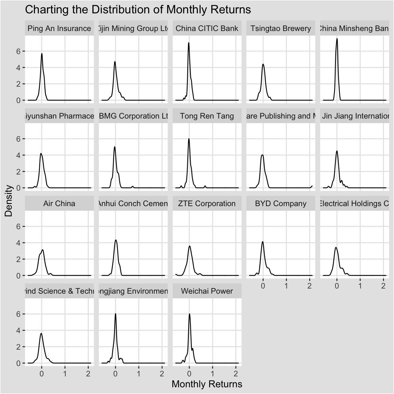
The plots where the peaks are low and spread out over a wide distance are riskier since their monthly returns tend to fluctuate more often between negative and positive and are less likely to be similar over long periods of time. The plots where the peak is high and nearer to positive returns are less risky. Air China appears to be riskiest, followed by Ekectrical Holdings. Banks appears to the least risky.
Analyzing the risk vs return
ggplot(Summary_monthly_returns,aes(x=Standard_Deviation,y=Mean))+
  geom_point()+
  ggrepel::geom_text_repel(position="identity",label=Summary_monthly_returns$symbol)+
  theme_solarized()+
  labs(x="Risk",
       y="Expected Monthly Return",
       title = "Charting the Risk vs. Expected Return of stocks")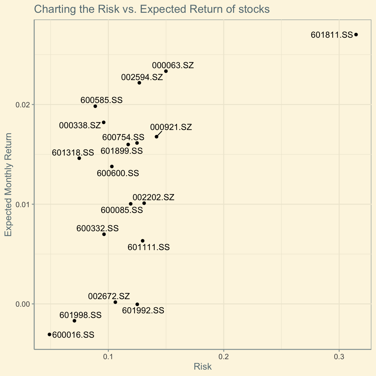
Boxplot of annual returns
myStocks_returns_annual %>%
  group_by(name) %>%
  mutate(median_return= median(yearly.returns)) %>%

  # arrange stocks by median yearly return, so highest median return appears first, etc.
  ggplot(aes(x=reorder(name, median_return), y=yearly.returns, colour=name)) +
  geom_boxplot()+
  coord_flip()+
  labs(x="Stock",
       y="Returns",
       title = "Boxplot of Annual Returns")+
  scale_y_continuous(labels = scales::percent_format(accuracy = 2))+
  guides(color=FALSE) +
  theme_bw()+
  NULL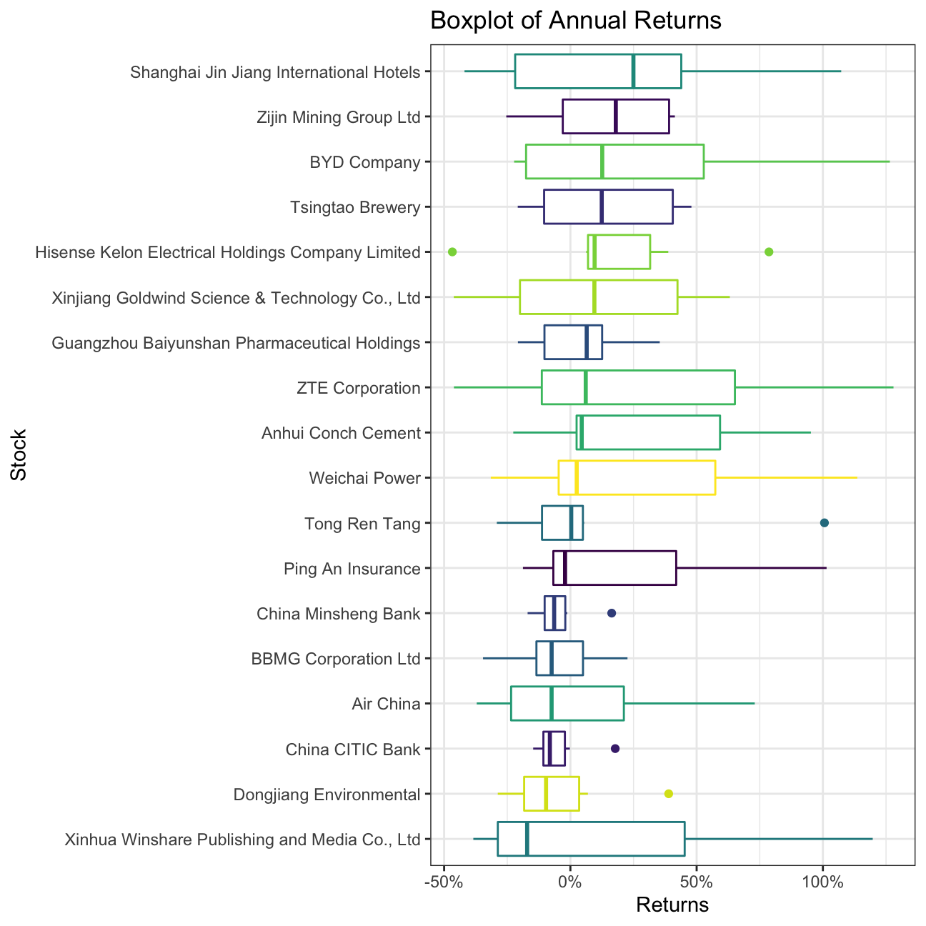
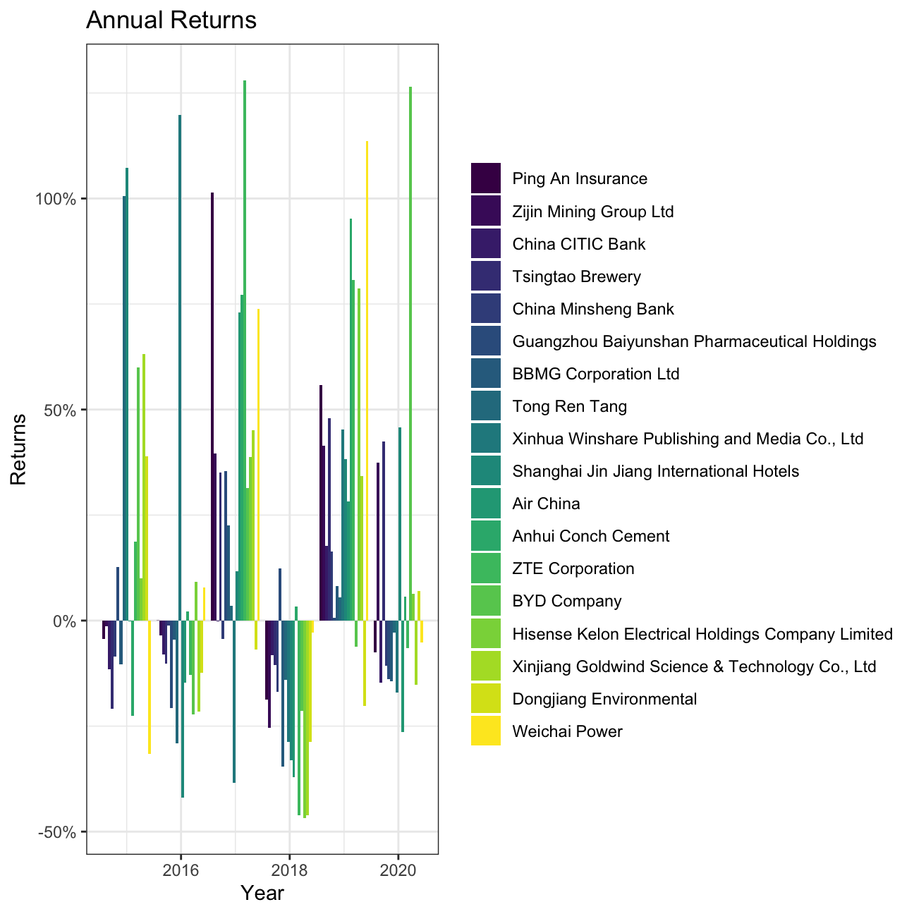
Bar plot that shows return for each stock on a year-by-year basis
ggplot(myStocks_returns_annual, aes(x=year(date), y=yearly.returns, fill=name)) +
  geom_col(position = "dodge")+
  labs(x="Year", y="Returns", title = "Annual Returns")+
  scale_y_continuous(labels = scales::percent)+
  guides(fill=guide_legend(title=NULL))+
  theme_bw()+
  NULL